Introduction to Clay Foundation Model for Earth Observation

• Clay is masked autoencoder based model that was training using satellite sensors such as Sentinel-2, Sentinel-1, Landsat, NAIP, MODIS, among others, in a self-supervised approach.

• This model supports any number of bands, which makes it practical on the band selection for specific application, as not all bands are useful for all kinds of applications.

• As in any transformer-based autoencoder, the Clay model consists of 3 components:

  • Embedding block: which generates embeddings from the input images and the wavelengths of the bands involved.

  • Positional encoding: which encodes spatial and temporal information by adding positional encoding to the model. This encoding is scaled according to the Ground Sampling Distance and combined with location information (lat/lon) and time step (week/hour).

  • Masked autoencoder: A VIT-based MAE which is used to reconstruct the sensor data for all bands. It is associated with 95% of the loss, which is known as the construction loss.

  • Teacher: DINOv2 is used as a teacher to compute the representation loss, which accounts for the remaining 5% of the total loss.

Use case: Unsupervised change detection in Earth Observation with Sentinel-1 and Sentinel-2 data

• The Clay foundation model is fed patches of these images, each patch of size 256x256 and the number of bands (2 for Sentinel-1 and 4 for Sentinel-2).

• The model also takes information about the coordinates of the center of the patch, sensor name, timestamp of the acquisition of the scene, wavelength of the involved bands, and Ground Sampling Distance of the sensor.

• The model estimates embeddings of each patch. These embeddings can be organized to be of size 1024x32x32.

• Pixel-wise distance functions are then used to compute a difference map between pre- and post-event image embeddings.

• The results of the patches are stitched.

• The resulting difference map is then scaled up to be of the size of the input image.

Getting Started

Download the model weights inside the clay folder from Clay v1.5

!wget -O ./clay/clay-v1.5.ckpt "https://huggingface.co/made-with-clay/Clay/resolve/main/v1.5/clay-v1.5.ckpt?download=true"

--2025-06-23 15:05:13--  https://huggingface.co/made-with-clay/Clay/resolve/main/v1.5/clay-v1.5.ckpt?download=true
Resolving huggingface.co (huggingface.co)... 3.165.190.15, 3.165.190.19, 3.165.190.31, ...
Connecting to huggingface.co (huggingface.co)|3.165.190.15|:443... connected.
HTTP request sent, awaiting response... 302 Found
Location: https://cdn-lfs-us-1.hf.co/repos/9e/5f/9e5f70717de49e5e8fb94cc66c7c40e24e6800ae6dbf377099154c19eafdc5f6/21432069250b9b3f9a65ffd0071c5ad56b793247285ab0604edf7f531d4798d0?response-content-disposition=attachment%3B+filename*%3DUTF-8%27%27clay-v1.5.ckpt%3B+filename%3D%22clay-v1.5.ckpt%22%3B&Expires=1750687513&Policy=eyJTdGF0ZW1lbnQiOlt7IkNvbmRpdGlvbiI6eyJEYXRlTGVzc1RoYW4iOnsiQVdTOkVwb2NoVGltZSI6MTc1MDY4NzUxM319LCJSZXNvdXJjZSI6Imh0dHBzOi8vY2RuLWxmcy11cy0xLmhmLmNvL3JlcG9zLzllLzVmLzllNWY3MDcxN2RlNDllNWU4ZmI5NGNjNjZjN2M0MGUyNGU2ODAwYWU2ZGJmMzc3MDk5MTU0YzE5ZWFmZGM1ZjYvMjE0MzIwNjkyNTBiOWIzZjlhNjVmZmQwMDcxYzVhZDU2Yjc5MzI0NzI4NWFiMDYwNGVkZjdmNTMxZDQ3OThkMD9yZXNwb25zZS1jb250ZW50LWRpc3Bvc2l0aW9uPSoifV19&Signature=b0XR3ijYD3ub5pndiz5rOrlbTodBC0qWSiflGM5-yG%7EP8nYqG3zMNKi8heLzrzOf1peX655L0ZY2-qNahP0AjaGjoVbAPlL7z-v%7EzW2wGjhB-f5n3ARWaviEXyU9aJdJ9z-5KNFUYF-3sVJ-do6iherwj899Z7MbyMf--tQMonEKKI3OEW93eGSi3nOLvhq8SnZapDp25hcYrqjFBtZxgXEoq2yOGInnL00yQEoG7MNWqO0-O31eFVGhCUC%7E56qeoVfO8VyxqUFJz9bYZlJFgJG8mLSBmdxt8zMhFYwZ6o8ndew49C8qcTzPZURK2lw8t-9BsXRKZFSGE3IFYzhk6g__&Key-Pair-Id=K24J24Z295AEI9 [following]
--2025-06-23 15:05:13--  https://cdn-lfs-us-1.hf.co/repos/9e/5f/9e5f70717de49e5e8fb94cc66c7c40e24e6800ae6dbf377099154c19eafdc5f6/21432069250b9b3f9a65ffd0071c5ad56b793247285ab0604edf7f531d4798d0?response-content-disposition=attachment%3B+filename*%3DUTF-8%27%27clay-v1.5.ckpt%3B+filename%3D%22clay-v1.5.ckpt%22%3B&Expires=1750687513&Policy=eyJTdGF0ZW1lbnQiOlt7IkNvbmRpdGlvbiI6eyJEYXRlTGVzc1RoYW4iOnsiQVdTOkVwb2NoVGltZSI6MTc1MDY4NzUxM319LCJSZXNvdXJjZSI6Imh0dHBzOi8vY2RuLWxmcy11cy0xLmhmLmNvL3JlcG9zLzllLzVmLzllNWY3MDcxN2RlNDllNWU4ZmI5NGNjNjZjN2M0MGUyNGU2ODAwYWU2ZGJmMzc3MDk5MTU0YzE5ZWFmZGM1ZjYvMjE0MzIwNjkyNTBiOWIzZjlhNjVmZmQwMDcxYzVhZDU2Yjc5MzI0NzI4NWFiMDYwNGVkZjdmNTMxZDQ3OThkMD9yZXNwb25zZS1jb250ZW50LWRpc3Bvc2l0aW9uPSoifV19&Signature=b0XR3ijYD3ub5pndiz5rOrlbTodBC0qWSiflGM5-yG%7EP8nYqG3zMNKi8heLzrzOf1peX655L0ZY2-qNahP0AjaGjoVbAPlL7z-v%7EzW2wGjhB-f5n3ARWaviEXyU9aJdJ9z-5KNFUYF-3sVJ-do6iherwj899Z7MbyMf--tQMonEKKI3OEW93eGSi3nOLvhq8SnZapDp25hcYrqjFBtZxgXEoq2yOGInnL00yQEoG7MNWqO0-O31eFVGhCUC%7E56qeoVfO8VyxqUFJz9bYZlJFgJG8mLSBmdxt8zMhFYwZ6o8ndew49C8qcTzPZURK2lw8t-9BsXRKZFSGE3IFYzhk6g__&Key-Pair-Id=K24J24Z295AEI9
Resolving cdn-lfs-us-1.hf.co (cdn-lfs-us-1.hf.co)... 18.173.233.98, 18.173.233.39, 18.173.233.41, ...
Connecting to cdn-lfs-us-1.hf.co (cdn-lfs-us-1.hf.co)|18.173.233.98|:443... connected.
HTTP request sent, awaiting response... 200 OK
Length: 5158764629 (4,8G) [binary/octet-stream]
Saving to: ‘./clay/clay-v1.5.ckpt’

./clay/clay-v1.5.ck 100%[===================>]   4,80G  38,1MB/s    in 96s     

2025-06-23 15:06:50 (51,0 MB/s) - ‘./clay/clay-v1.5.ckpt’ saved [5158764629/5158764629]

Import libraries

import sys
sys.path.append("./clay")
import random
import math
from tqdm import tqdm
import requests
from tqdm import tqdm
import geopandas as gpd
import numpy as np
import pandas as pd
import pystac_client
import stackstac
import torch
import yaml
from box import Box
from matplotlib import pyplot as plt
import rasterio
from rasterio.enums import Resampling
from pyproj import Transformer
from shapely import Point
from torchvision.transforms import v2
from clay.src.module import ClayMAEModule
import torch
import torch.nn.functional as F
from torch.utils.data import Dataset, DataLoader
from scipy.ndimage import zoom
import planetary_computer
import folium
from utils import (
    reconstruct_image_from_patches,
    pixelwise_cosine_distance_npy,
    pixelwise_cosine_distance_torch,
    normalize_latlon,
    normalize_timestamp,
    denormalize_images,
    rearrange_embeddings
)

Define variables

LAT, LON = 39.3336, -0.3545
START_DATE_S2 = "2024-10-01"
END_DATE_S2 = "2024-12-01"
AWS_STAC_API = "https://earth-search.aws.element84.com/v1"
COLLECTION_S2 = "sentinel-2-l2a"
BEFORE_DATE_S2 = "2024-10-01"
AFTER_DATE_S2 = "2024-11-10"
PLANETARY_TOKEN_URL = "https://planetarycomputer.microsoft.com/api/sas/v1/token"
PLANETARY_STAC_API = "https://planetarycomputer.microsoft.com/api/stac/v1"
COLLECTION_S1 = "sentinel-1-rtc"
START_DATE_S1 = "2024-10-01"
END_DATE_S1 = "2024-12-01"
BEFORE_DATE_S1 = "2024-10-07"
AFTER_DATE_S1 = "2024-11-12"
PATCH_SIZE = 256
STRIDE = 256
DEVICE = "mps" if torch.mps.is_available() else "cuda" if torch.cuda.is_available() else "cpu"

Change Detection Using Sentinel-2 Images

Search for Sentinel-2 Images

catalog = pystac_client.Client.open(AWS_STAC_API)
search = catalog.search(
    collections=[COLLECTION_S2],
    datetime=f"{START_DATE_S2}/{END_DATE_S2}",
    bbox=(LON - 1e-3, LAT - 1e-3, LON + 1e-3, LAT + 1e-3),
    max_items=100,
    query={"eo:cloud_cover": {"lt": 50}},
)

all_items = search.get_all_items()

# Reduce to one per date (there might be some duplicates
# based on the location)
items = []
dates = []
for item in all_items:
    item_date = item.datetime
    if item_date.date() not in dates and (item_date.isoformat()[0:10] == BEFORE_DATE_S2 or item_date.isoformat()[0:10] == AFTER_DATE_S2) :
        items.append(item)
        dates.append(item.datetime.date())

print(f"Found {len(items)} items")

/Users/syam/virtualenvs/myvenv/lib/python3.13/site-packages/pystac_client/item_search.py:896: FutureWarning: get_all_items() is deprecated, use item_collection() instead.
  warnings.warn(

Found 2 items

Create a bounding box around the POI

epsg = items[0].properties["proj:code"]
poidf = gpd.GeoDataFrame(
    pd.DataFrame(),
    crs="EPSG:4326",
    geometry=[Point(LON, LAT)],
).to_crs(epsg)
coords = poidf.iloc[0].geometry.coords[0]
size = 2048
gsd = 10
bounds = (
    coords[0] - (size * gsd) // 2,
    coords[1] - (size * gsd) // 2,
    coords[0] + (size * gsd) // 2,
    coords[1] + (size * gsd) // 2,
)

Get the Sentinel-2 data using StackStac

stack = stackstac.stack(
    items,
    bounds=bounds,
    snap_bounds=False,
    epsg=int(epsg.split(":")[-1]),
    resolution=gsd,
    dtype="float64",
    rescale=False,
    fill_value=0,
    assets=["blue", "green", "red", "nir", "rededge2", "swir16"],
    resampling=Resampling.nearest,
)

stack = stack.compute()

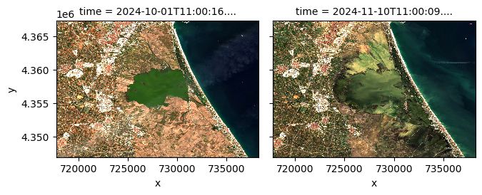
Visualize Sentinel-2 data

stack.sel(band=["red", "green", "blue"]).plot.imshow(
    row="time", rgb="band", vmin=0, vmax=2000, col_wrap=6
)

<xarray.plot.facetgrid.FacetGrid at 0x17da86270>

Prepare metadata required by the model and data transformation pipeline

platform = "sentinel-2-l2a"
metadata = Box(yaml.safe_load(open("./clay/configs/metadata.yaml")))
mean = []
std = []
waves = []
for band in stack.band:
    mean.append(metadata[platform].bands.mean[str(band.values)])
    std.append(metadata[platform].bands.std[str(band.values)])
    waves.append(metadata[platform].bands.wavelength[str(band.values)])

transform = v2.Compose(
    [
        v2.Normalize(mean=mean, std=std),
    ]
)

print (mean)
print (std)
print (waves)

[1105.0, 1355.0, 1552.0, 2743.0, 2422.0, 2388.0]
[1809.0, 1757.0, 1888.0, 1742.0, 1732.0, 1470.0]
[0.493, 0.56, 0.665, 0.842, 0.74, 1.61]

Create patches from the Sentinel-2 images of size 256x256

pixels_before = torch.from_numpy(stack.sel(time="2024-10-01").data.astype(np.float32))
print (pixels_before.shape)
batch_size, bands, height, width = pixels_before.shape
patches_before = F.unfold(
    pixels_before, kernel_size=PATCH_SIZE, stride=STRIDE
)  # (BATCH, BANDS*PATCH_SIZE*PATCH_SIZE, NUM_PATCHES)
patches_before = patches_before.permute(0, 2, 1)  # (BATCH, NUM_PATCHES, BANDS*PATCH_SIZE*PATCH_SIZE)
patches_before = patches_before.view(
    batch_size, -1, bands, PATCH_SIZE, PATCH_SIZE
)  # (BATCH, NUM_PATCHES, BANDS, PATCH_SIZE, PATCH_SIZE)
patches_before = patches_before.reshape(-1, bands, PATCH_SIZE, PATCH_SIZE)
print(patches_before.shape)

torch.Size([1, 6, 2048, 2048])
torch.Size([64, 6, 256, 256])

pixels_after = torch.from_numpy(stack.sel(time="2024-11-10").data.astype(np.float32))
print(pixels_after.shape)
batch_size, bands, height, width = pixels_after.shape
patches_after = F.unfold(
    pixels_after, kernel_size=PATCH_SIZE, stride=STRIDE
)  # (BATCH, BANDS*PATCH_SIZE*PATCH_SIZE, NUM_PATCHES)
patches_after = patches_after.permute(
    0, 2, 1
)  # (BATCH, NUM_PATCHES, BANDS*PATCH_SIZE*PATCH_SIZE)
patches_after = patches_after.view(
    batch_size, -1, bands, PATCH_SIZE, PATCH_SIZE
)  # (BATCH, NUM_PATCHES, BANDS, PATCH_SIZE, PATCH_SIZE)
patches_after = patches_after.reshape(-1, bands, PATCH_SIZE, PATCH_SIZE)
print(patches_after.shape)

torch.Size([1, 6, 2048, 2048])
torch.Size([64, 6, 256, 256])

Get centers and timestamps for the image patches

x_coords = stack.coords["x"].values
y_coords = stack.coords["y"].values
time_values = stack.coords["time"].values.astype("datetime64[s]")
img_id_values = stack.id.values
height, width = pixels_before.shape[-2:]  # Get spatial dimensions
patch_centers_x_idx = np.arange(PATCH_SIZE // 2, width, STRIDE)  # X indices of centers
patch_centers_y_idx = np.arange(PATCH_SIZE // 2, height, STRIDE)  # Y indices of centers

center_x_grid, center_y_grid = np.meshgrid(patch_centers_x_idx, patch_centers_y_idx)
center_x_coords = x_coords[center_x_grid]  # Map X indices to coordinates
center_y_coords = y_coords[center_y_grid]  # Map Y indices to coordinates

patch_centers = np.stack([center_x_coords.ravel(), center_y_coords.ravel()], axis=-1)
num_patches = len(patch_centers)
patches_per_image = num_patches // 18
timesteps_patches = (
    np.repeat(time_values, num_patches).astype("datetime64[ms]").tolist()
)
img_id_patches = np.repeat(img_id_values, num_patches).tolist()
original_crs = stack.attrs["crs"]  # Assuming you are using a rioxarray-enabled dataset
target_crs = "EPSG:4326"  # WGS 84
transformer = Transformer.from_crs(original_crs, target_crs, always_xy=True)
x_coords = patch_centers[:, 0]
y_coords = patch_centers[:, 1]
lon, lat = transformer.transform(x_coords, y_coords)
patch_centers_epsg4326 = np.stack([lon, lat], axis=-1)
patch_centers_epsg4326_all = np.array([patch_centers_epsg4326] * batch_size).reshape(
    batch_size * num_patches, 2
)

Visualize the patch centers on a map

# Initialize a folium map centered at the average location of your patch centers
map_center = [
    np.mean([coord[1] for coord in patch_centers_epsg4326[0:64]]),  # Average latitude
    np.mean([coord[0] for coord in patch_centers_epsg4326[0:64]]),  # Average longitude
]

m = folium.Map(location=map_center, zoom_start=10)

# Add a circle marker for each patch center
for lon, lat in patch_centers_epsg4326[0:64]:
    folium.CircleMarker(
        location=[lat, lon],  # Note: folium uses (lat, lon)
        radius=5,  # Marker size
        color="blue",
        fill=True,
        fill_color="blue",
        fill_opacity=0.6,
    ).add_to(m)
m

Make this Notebook Trusted to load map: File -> Trust Notebook

Normalize timestamps and coordinates as required by the model

times = [normalize_timestamp(dat) for dat in timesteps_patches]
week_norm = [dat[0] for dat in times]
hour_norm = [dat[1] for dat in times]
latlons = [normalize_latlon(lat, lon) for lat, lon in patch_centers_epsg4326_all]
lat_norm = [dat[0] for dat in latlons]
lon_norm = [dat[1] for dat in latlons]

Transform the data

transformed_patches_before = transform(patches_before)
transformed_patches_after = transform(patches_after)

Initialize the model

ckpt = "./clay/clay-v1.5.ckpt"
torch.set_default_device(DEVICE)
model = ClayMAEModule.load_from_checkpoint(
    ckpt,
    model_size="large",
    metadata_path="./clay/configs/metadata.yaml",
    dolls=[16, 32, 64, 128, 256, 768, 1024],
    doll_weights=[1, 1, 1, 1, 1, 1, 1],
    mask_ratio=0.0,
    shuffle=False,
)
model.eval()
model = model.to(DEVICE)

Inference on the before image

before_embeddings = []
m_batch_size = 16
for start_idx in tqdm(
    range(0, transformed_patches_before.size(0), m_batch_size),
    desc="Processing batches",
):
    end_idx = min(start_idx + m_batch_size, transformed_patches_before.size(0))
    datacube = {
        "platform": platform,
        "time": torch.tensor(
            np.hstack((week_norm[start_idx:end_idx], hour_norm[start_idx:end_idx])),
            dtype=torch.float32,
            device=DEVICE,
        ),
        "latlon": torch.tensor(
            np.hstack((lat_norm[start_idx:end_idx], lon_norm[start_idx:end_idx])),
            dtype=torch.float32,
            device=DEVICE,
        ),
        "pixels": transformed_patches_before[start_idx:end_idx].to(DEVICE),
        "gsd": torch.tensor(
            [metadata[platform].gsd], dtype=torch.float32, device=DEVICE
        ),
        "waves": torch.tensor(waves, device=DEVICE),
    }
    with torch.no_grad():
        unmsk_patch, unmsk_idx, msk_idx, msk_matrix = model.model.encoder(datacube)
        before_embeddings.append(unmsk_patch)

Processing batches: 100%|██████████| 4/4 [00:16<00:00,  4.16s/it]

Inference on the after image

after_embeddings = []
m_batch_size = 16
for start_idx in tqdm(
    range(0, transformed_patches_after.size(0), m_batch_size),
    desc="Processing batches",
):
    end_idx = min(start_idx + m_batch_size, transformed_patches_after.size(0))
    datacube = {
        "platform": platform,
        "time": torch.tensor(
            np.hstack((week_norm[start_idx+64:end_idx+64], hour_norm[start_idx+64:end_idx+64])),
            dtype=torch.float32,
            device=DEVICE,
        ),
        "latlon": torch.tensor(
            np.hstack((lat_norm[start_idx:end_idx], lon_norm[start_idx:end_idx])),
            dtype=torch.float32,
            device=DEVICE,
        ),
        "pixels": transformed_patches_after[start_idx:end_idx].to(DEVICE),
        "gsd": torch.tensor(
            [metadata[platform].gsd], dtype=torch.float32, device=DEVICE
        ),
        "waves": torch.tensor(waves, device=DEVICE),
    }
    with torch.no_grad():
        unmsk_patch, unmsk_idx, msk_idx, msk_matrix = model.model.encoder(datacube)
        after_embeddings.append(unmsk_patch)

Processing batches: 100%|██████████| 4/4 [00:16<00:00,  4.06s/it]

Flatten the lists containing the image embeddings

flattened_before_embeddings = torch.cat(before_embeddings, dim=0)
flattened_after_embeddings = torch.cat(after_embeddings, dim=0)
print (flattened_before_embeddings.shape)
print (flattened_after_embeddings.shape)

torch.Size([64, 1025, 1024])
torch.Size([64, 1025, 1024])

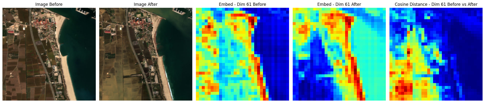
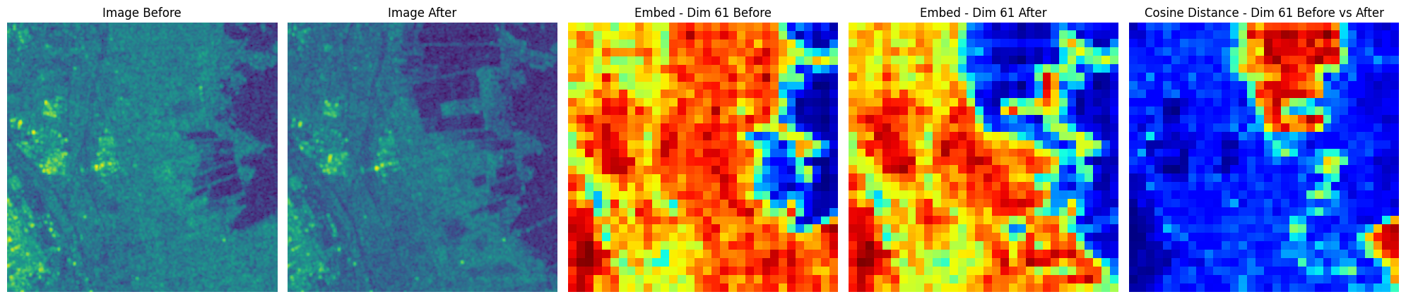
Visualize an example

patch_id = np.random.randint(0,transformed_patches_before.shape[0])
print(f"Patch ID: {patch_id}")
embed_id = (
    61  # random.sample(range(1024), 4) # [61,62,63,64]  # pick any embedding dimensions
)
img_before = transformed_patches_before[patch_id].detach().cpu().numpy()
img_after = transformed_patches_after[patch_id].detach().cpu().numpy()
embedding_before = flattened_before_embeddings[patch_id]
embedding_after = flattened_after_embeddings[patch_id]
img_before = denormalize_images(img_before, mean, std)
img_before = (img_before / 10000).astype(np.float32)
img_after = denormalize_images(img_after, mean, std)
img_after = (img_after / 10000).astype(np.float32)
unmsk_embed_before = rearrange_embeddings(embedding_before.unsqueeze(0))
unmsk_embed_after = rearrange_embeddings(embedding_after.unsqueeze(0))
fig, axs = plt.subplots(1, 5, figsize=(20, 14))
axs[0].imshow(img_before[0, [2, 1, 0], ...].transpose(1, 2, 0) * 2.5)
axs[0].set_axis_off()
axs[0].set_title(f"Image Before")
axs[1].imshow(img_after[0, [2, 1, 0], ...].transpose(1, 2, 0) * 2.5)
axs[1].set_axis_off()
axs[1].set_title(f"Image After")
axs[2].imshow(unmsk_embed_before[0, embed_id], cmap="jet")
axs[2].set_axis_off()
axs[2].set_title(f"Embed - Dim {embed_id} Before")
axs[3].imshow(unmsk_embed_after[0, embed_id], cmap="jet")
axs[3].set_axis_off()
axs[3].set_title(f"Embed - Dim {embed_id} After")
axs[4].imshow(
    pixelwise_cosine_distance_npy(
        unmsk_embed_before,unmsk_embed_after
    )[0],
    cmap="jet",
)
axs[4].set_axis_off()
axs[4].set_title(f"Cosine Distance - Dim {embed_id} Before vs After")
plt.tight_layout()
plt.show()

Patch ID: 4

Clipping input data to the valid range for imshow with RGB data ([0..1] for floats or [0..255] for integers). Got range [7.629394e-09..1.411].
Clipping input data to the valid range for imshow with RGB data ([0..1] for floats or [0..255] for integers). Got range [0.0002499907..4.4579997].

Rearrange embeddings, compute difference matrix and interpolate to original patch size

re_after_embeddings = rearrange_embeddings(flattened_after_embeddings)
re_before_embeddings = rearrange_embeddings(flattened_before_embeddings)
diff = pixelwise_cosine_distance_torch(torch.from_numpy(re_after_embeddings), torch.from_numpy(re_before_embeddings))
print(diff.shape)

torch.Size([64, 32, 32])

diff = F.interpolate(
    diff.unsqueeze(1), size=(256, 256), mode="bilinear", align_corners=False
)
print (diff.shape)

torch.Size([64, 1, 256, 256])

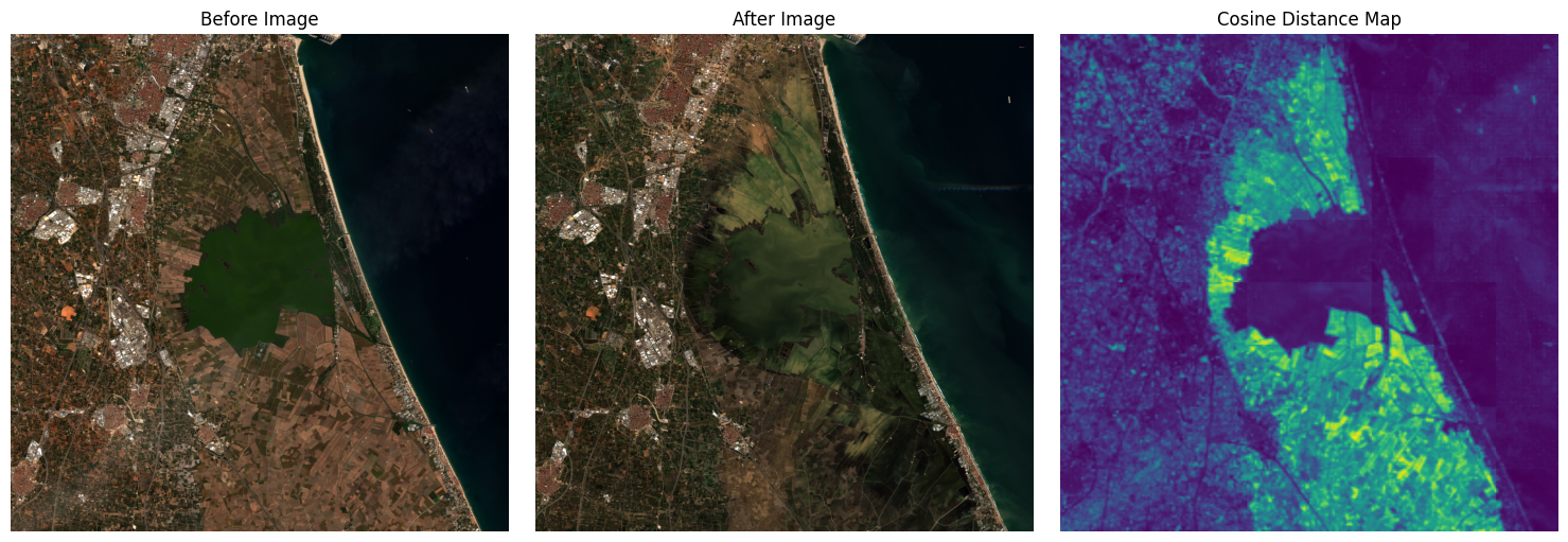
Reconstruct diff in original image size and visualize

diff = diff.to(DEVICE)
recon_diff = reconstruct_image_from_patches(
    diff, (2048, 2048), PATCH_SIZE, STRIDE, channels=1
)

pixels_before_rgb = pixels_before[0, [2, 1, 0], :, :].cpu().numpy()/10000.0
pixels_after_rgb = pixels_after[0, [2, 1, 0], :, :].cpu().numpy()/10000.0

pixels_before_rgb = np.transpose(pixels_before_rgb, (1, 2, 0))
pixels_after_rgb = np.transpose(pixels_after_rgb, (1, 2, 0))

pixels_before_rgb = np.clip(pixels_before_rgb, 0, 1)
pixels_after_rgb = np.clip(pixels_after_rgb, 0, 1)


diff_map = recon_diff.squeeze(-1)

# Plotting
plt.figure(figsize=(15, 5))

plt.subplot(1, 3, 1)
plt.imshow(pixels_before_rgb*2.5)
plt.title("Before Image")
plt.axis("off")

plt.subplot(1, 3, 2)
plt.imshow(pixels_after_rgb*2.5)
plt.title("After Image")
plt.axis("off")

plt.subplot(1, 3, 3)
plt.imshow(diff_map, cmap="viridis")
plt.title("Cosine Distance Map")
plt.axis("off")

plt.tight_layout()
plt.show()

Clipping input data to the valid range for imshow with RGB data ([0..1] for floats or [0..255] for integers). Got range [0.0..2.5].
Clipping input data to the valid range for imshow with RGB data ([0..1] for floats or [0..255] for integers). Got range [0.0..2.5].

Change Detection Using Sentinel-1 Images

Search STAC API for Sentinel-1 images

response = requests.get(f"{PLANETARY_TOKEN_URL}/{COLLECTION_S1}")

if response.status_code == 200:
    response = response.json()  # Assuming the response contains a JSON object
    token = response["token"]
    headers ={"Authorization":f"Bearer {token}"}
else:
    print(f"Failed to get token. Status code: {response.status_code}")
    exit()

# Search the catalogue
catalog = pystac_client.Client.open(PLANETARY_STAC_API)
search = catalog.search(
    collections=[COLLECTION_S1],
    datetime=f"{START_DATE_S1}/{END_DATE_S1}",
    bbox=(LON - 1e-3, LAT - 1e-3, LON + 1e-3, LAT + 1e-3),
    )
all_items = search.get_all_items()
items = []
dates = []
for item in all_items:
    item_date = item.datetime
    if item_date.date() not in dates  and item.properties["sat:orbit_state"]=="ascending" and (item_date.isoformat()[0:10] == BEFORE_DATE_S1 or item_date.isoformat()[0:10] == AFTER_DATE_S1) :
        items.append(planetary_computer.sign_item(item))
        dates.append(item.datetime.date())

print(f"Found {len(items)} items")

/Users/syam/virtualenvs/myvenv/lib/python3.13/site-packages/pystac_client/item_search.py:896: FutureWarning: get_all_items() is deprecated, use item_collection() instead.
  warnings.warn(

Found 2 items

Create a bounding box around POI

# Extract coordinate system from first item
epsg = items[0].properties["proj:code"]

# Convert point of interest into the image projection
# (assumes all images are in the same projection)
poidf = gpd.GeoDataFrame(
    pd.DataFrame(),
    crs="EPSG:4326",
    geometry=[Point(LON, LAT)],
).to_crs(epsg)

coords = poidf.iloc[0].geometry.coords[0]

# Create bounds in projection
size = 2048
gsd = 10
bounds = (
    coords[0] - (size * gsd) // 2,
    coords[1] - (size * gsd) // 2,
    coords[0] + (size * gsd) // 2,
    coords[1] + (size * gsd) // 2,
)

Get the Sentinel-1 data using StackStac

stack = stackstac.stack(
    items,
    bounds=bounds,
    snap_bounds=False,
    epsg=int(epsg.split(":")[-1]),
    resolution=gsd,
    dtype="float64",
    rescale=False,
    # fill_value=np.nan,
    assets=["vv", "vh"],
    resampling=Resampling.nearest,
)
stack = stack.compute()

Convert Sentinel-1 data from linear intensity to decibel (dB)

eps = 1e-10
stack_db = 10 * np.log10(stack + eps)

Visualize Sentinel-1 data

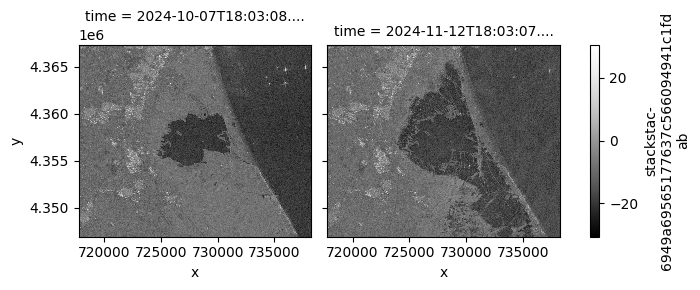
stack_db.sel(band="vv").plot.imshow(
    row="time",
    col_wrap=2,
    cmap=plt.cm.Greys_r,
)

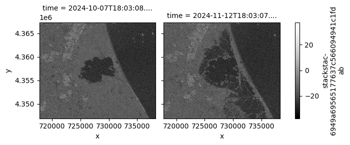
# Plot VH Band with its own scaling
stack_db.sel(band="vh").plot.imshow(
    row="time",
    col_wrap=2,
    cmap=plt.cm.Greys_r,
)

plt.show()

Prepare metadata required for the model and the transformation pipeline

# Extract mean, std, and wavelengths from metadata
platform = "sentinel-1-rtc"
metadata = Box(yaml.safe_load(open("./clay/configs/metadata.yaml")))
mean = []
std = []
waves = []
# Use the band names to get the correct values in the correct order.
for band in stack_db.band:
    mean.append(metadata[platform].bands.mean[str(band.values)])
    std.append(metadata[platform].bands.std[str(band.values)])
    waves.append(metadata[platform].bands.wavelength[str(band.values)])

# Prepare the normalization transform function using the mean and std values.
transform = v2.Compose(
    [
        v2.Normalize(mean=mean, std=std),
    ]
)

pixels_before = torch.from_numpy(stack_db.sel(time="2024-10-07").data.astype(np.float32))
print(pixels_before.shape)
batch_size, bands, height, width = pixels_before.shape
patches_before = F.unfold(
    pixels_before, kernel_size=PATCH_SIZE, stride=STRIDE
)  # (BATCH, BANDS*PATCH_SIZE*PATCH_SIZE, NUM_PATCHES)
patches_before = patches_before.permute(
    0, 2, 1
)  # (BATCH, NUM_PATCHES, BANDS*PATCH_SIZE*PATCH_SIZE)
patches_before = patches_before.view(
    batch_size, -1, bands, PATCH_SIZE, PATCH_SIZE
)  # (BATCH, NUM_PATCHES, BANDS, PATCH_SIZE, PATCH_SIZE)
patches_before = patches_before.reshape(-1, bands, PATCH_SIZE, PATCH_SIZE)
print(patches_before.shape)

torch.Size([1, 2, 2048, 2048])
torch.Size([64, 2, 256, 256])

pixels_after = torch.from_numpy(stack_db.sel(time="2024-11-12").data.astype(np.float32))
print(pixels_after.shape)
batch_size, bands, height, width = pixels_after.shape
patches_after = F.unfold(
    pixels_after, kernel_size=PATCH_SIZE, stride=STRIDE
)  # (BATCH, BANDS*PATCH_SIZE*PATCH_SIZE, NUM_PATCHES)
patches_after = patches_after.permute(
    0, 2, 1
)  # (BATCH, NUM_PATCHES, BANDS*PATCH_SIZE*PATCH_SIZE)
patches_after = patches_after.view(
    batch_size, -1, bands, PATCH_SIZE, PATCH_SIZE
)  # (BATCH, NUM_PATCHES, BANDS, PATCH_SIZE, PATCH_SIZE)
patches_after = patches_after.reshape(-1, bands, PATCH_SIZE, PATCH_SIZE)
print(patches_after.shape)

torch.Size([1, 2, 2048, 2048])
torch.Size([64, 2, 256, 256])

Get centers and timestamps of the patches

x_coords = stack_db.coords["x"].values
y_coords = stack_db.coords["y"].values
time_values = stack_db.coords["time"].values.astype("datetime64[s]")
img_id_values = stack_db.id.values
height, width = pixels_before.shape[-2:]  # Get spatial dimensions
patch_centers_x_idx = np.arange(PATCH_SIZE // 2, width, STRIDE)  # X indices of centers
patch_centers_y_idx = np.arange(PATCH_SIZE // 2, height, STRIDE)  # Y indices of centers

center_x_grid, center_y_grid = np.meshgrid(patch_centers_x_idx, patch_centers_y_idx)
center_x_coords = x_coords[center_x_grid]  # Map X indices to coordinates
center_y_coords = y_coords[center_y_grid]  # Map Y indices to coordinates

patch_centers = np.stack([center_x_coords.ravel(), center_y_coords.ravel()], axis=-1)
num_patches = len(patch_centers)
patches_per_image = num_patches // 18
timesteps_patches = (
    np.repeat(time_values, num_patches).astype("datetime64[ms]").tolist()
)
img_id_patches = np.repeat(img_id_values, num_patches).tolist()
original_crs = stack.attrs["crs"]  # Assuming you are using a rioxarray-enabled dataset
target_crs = "EPSG:4326"  # WGS 84
transformer = Transformer.from_crs(original_crs, target_crs, always_xy=True)
x_coords = patch_centers[:, 0]
y_coords = patch_centers[:, 1]
lon, lat = transformer.transform(x_coords, y_coords)
patch_centers_epsg4326 = np.stack([lon, lat], axis=-1)
patch_centers_epsg4326_all = np.array([patch_centers_epsg4326] * batch_size).reshape(
    batch_size * num_patches, 2
)

# Initialize a folium map centered at the average location of your patch centers
map_center = [
    np.mean([coord[1] for coord in patch_centers_epsg4326[0:64]]),  # Average latitude
    np.mean([coord[0] for coord in patch_centers_epsg4326[0:64]]),  # Average longitude
]

m = folium.Map(location=map_center, zoom_start=10)

# Add a circle marker for each patch center
for lon, lat in patch_centers_epsg4326[0:64]:
    folium.CircleMarker(
        location=[lat, lon],  # Note: folium uses (lat, lon)
        radius=5,  # Marker size
        color="blue",
        fill=True,
        fill_color="blue",
        fill_opacity=0.6,
    ).add_to(m)
m

Make this Notebook Trusted to load map: File -> Trust Notebook

Normalize timestamps and coordinates

times = [normalize_timestamp(dat) for dat in timesteps_patches]
week_norm = [dat[0] for dat in times]
hour_norm = [dat[1] for dat in times]
latlons = [normalize_latlon(lat, lon) for lat, lon in patch_centers_epsg4326_all]
lat_norm = [dat[0] for dat in latlons]
lon_norm = [dat[1] for dat in latlons]

Transform Sentinel-1 data

transformed_patches_before = transform(patches_before)
transformed_patches_after = transform(patches_after)

Inference on the before image

before_embeddings = []
m_batch_size = 16
for start_idx in tqdm(
    range(0, transformed_patches_before.size(0), m_batch_size),
    desc="Processing batches",
):
    end_idx = min(start_idx + m_batch_size, transformed_patches_before.size(0))
    datacube = {
        "platform": platform,
        "time": torch.tensor(
            np.hstack((week_norm[start_idx:end_idx], hour_norm[start_idx:end_idx])),
            dtype=torch.float32,
            device=DEVICE,
        ),
        "latlon": torch.tensor(
            np.hstack((lat_norm[start_idx:end_idx], lon_norm[start_idx:end_idx])),
            dtype=torch.float32,
            device=DEVICE,
        ),
        "pixels": transformed_patches_before[start_idx:end_idx].to(DEVICE),
        "gsd": torch.tensor(
            [metadata[platform].gsd], dtype=torch.float32, device=DEVICE
        ),
        "waves": torch.tensor(waves, device=DEVICE),
    }
    with torch.no_grad():
        unmsk_patch, unmsk_idx, msk_idx, msk_matrix = model.model.encoder(datacube)
        before_embeddings.append(unmsk_patch)

Processing batches: 100%|██████████| 4/4 [00:21<00:00,  5.28s/it]

Inference on the after image

after_embeddings = []
m_batch_size = 16
for start_idx in tqdm(
    range(0, transformed_patches_after.size(0), m_batch_size),
    desc="Processing batches",
):
    end_idx = min(start_idx + m_batch_size, transformed_patches_after.size(0))
    datacube = {
        "platform": platform,
        "time": torch.tensor(
            np.hstack(
                (
                    week_norm[start_idx + 64 : end_idx + 64],
                    hour_norm[start_idx + 64 : end_idx + 64],
                )
            ),
            dtype=torch.float32,
            device=DEVICE,
        ),
        "latlon": torch.tensor(
            np.hstack((lat_norm[start_idx:end_idx], lon_norm[start_idx:end_idx])),
            dtype=torch.float32,
            device=DEVICE,
        ),
        "pixels": transformed_patches_after[start_idx:end_idx].to(DEVICE),
        "gsd": torch.tensor(
            [metadata[platform].gsd], dtype=torch.float32, device=DEVICE
        ),
        "waves": torch.tensor(waves, device=DEVICE),
    }
    with torch.no_grad():
        unmsk_patch, unmsk_idx, msk_idx, msk_matrix = model.model.encoder(datacube)
        after_embeddings.append(unmsk_patch)

Processing batches: 100%|██████████| 4/4 [00:17<00:00,  4.25s/it]

Flatten the lists containing the embeddings

flattened_before_embeddings = torch.cat(before_embeddings, dim=0)
flattened_after_embeddings = torch.cat(after_embeddings, dim=0)
print(flattened_before_embeddings.shape)
print(flattened_after_embeddings.shape)

torch.Size([64, 1025, 1024])
torch.Size([64, 1025, 1024])

Visualize an example

patch_id = np.random.randint(0, transformed_patches_before.shape[0])
print(f"Patch ID: {patch_id}")
embed_id = (
    61  # random.sample(range(1024), 4) # [61,62,63,64]  # pick any embedding dimensions
)
img_before = transformed_patches_before[patch_id].detach().cpu().numpy()
img_after = transformed_patches_after[patch_id].detach().cpu().numpy()
embedding_before = flattened_before_embeddings[patch_id]
embedding_after = flattened_after_embeddings[patch_id]
img_before = denormalize_images(img_before, mean, std)
img_before = (img_before / 10000).astype(np.float32)
img_after = denormalize_images(img_after, mean, std)
img_after = (img_after / 10000).astype(np.float32)
unmsk_embed_before = rearrange_embeddings(embedding_before.unsqueeze(0))
unmsk_embed_after = rearrange_embeddings(embedding_after.unsqueeze(0))
fig, axs = plt.subplots(1, 5, figsize=(20, 14))
axs[0].imshow(img_before[0,0, ...])
axs[0].set_axis_off()
axs[0].set_title(f"Image Before")
axs[1].imshow(img_after[0, 0, ...])
axs[1].set_axis_off()
axs[1].set_title(f"Image After")
axs[2].imshow(unmsk_embed_before[0, embed_id], cmap="jet")
axs[2].set_axis_off()
axs[2].set_title(f"Embed - Dim {embed_id} Before")
axs[3].imshow(unmsk_embed_after[0, embed_id], cmap="jet")
axs[3].set_axis_off()
axs[3].set_title(f"Embed - Dim {embed_id} After")
axs[4].imshow(
    pixelwise_cosine_distance_npy(unmsk_embed_before, unmsk_embed_after)[0],
    cmap="jet",
)
axs[4].set_axis_off()
axs[4].set_title(f"Cosine Distance - Dim {embed_id} Before vs After")
plt.tight_layout()
plt.show()

Patch ID: 34

Rearrange embeddings, compute distance matrix and interpolate

re_after_embeddings = rearrange_embeddings(flattened_after_embeddings)
re_before_embeddings = rearrange_embeddings(flattened_before_embeddings)
diff = pixelwise_cosine_distance_torch(torch.from_numpy(re_after_embeddings), torch.from_numpy(re_before_embeddings))
print(diff.shape)

torch.Size([64, 32, 32])

diff = F.interpolate(
    diff.unsqueeze(1), size=(256, 256), mode="bilinear", align_corners=False
)
print(diff.shape)

torch.Size([64, 1, 256, 256])

Reconstruct the diff in original image size and visualize

diff = diff.to(DEVICE)
recon_diff = reconstruct_image_from_patches(
    diff, (2048, 2048), PATCH_SIZE, STRIDE, channels=1
)

def min_max_normalize(image):
    normalized = np.zeros_like(image)
    for band in range(image.shape[0]):
        band_min = image[band].min()
        band_max = image[band].max()
        normalized[band] = (image[band] - band_min) / (band_max - band_min + 1e-10)
    return normalized


pixels_before_np = pixels_before[0, :, :, :].cpu().numpy()  # shape: (2, H, W)
pixels_after_np = pixels_after[0, :, :, :].cpu().numpy()   # shape: (2, H, W)

pixels_before_np = min_max_normalize(pixels_before_np)
pixels_after_np = min_max_normalize(pixels_after_np)

# Create pseudo-RGB images by assigning band 0 -> R, band 1 -> G, and zero to B
H, W = pixels_before_np.shape[1], pixels_before_np.shape[2]

pixels_before_rgb = np.stack(
    [
        pixels_before_np[0],  # Red
        pixels_before_np[1],  # Green
        np.zeros((H, W)),  # Blue
    ],
    axis=-1,
)

pixels_after_rgb = np.stack(
    [pixels_after_np[0], pixels_after_np[1], np.zeros((H, W))],  # Red  # Green  # Blue
    axis=-1,
)

# Clip to [0, 1] for display
# pixels_before_rgb = np.clip(pixels_before_rgb, 0, 1)
# pixels_after_rgb = np.clip(pixels_after_rgb, 0, 1)

# Assuming diff_map is (H, W) or (H, W, 1)
diff_map = recon_diff.squeeze()
if diff_map.ndim == 3:
    diff_map = diff_map.squeeze(-1)

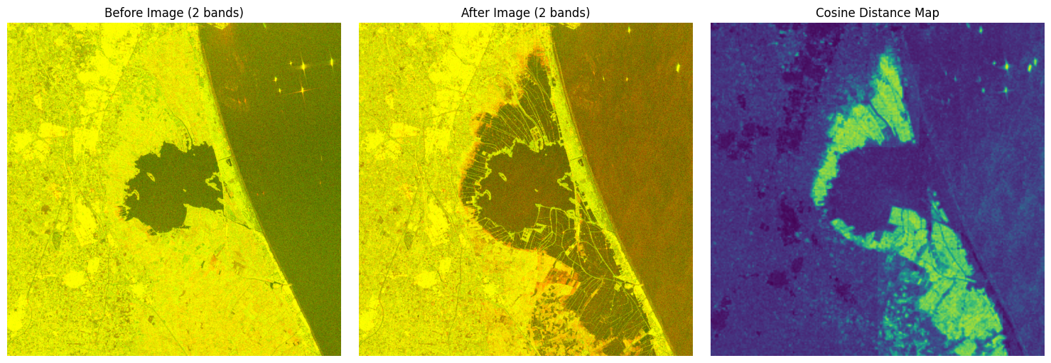
# Plotting
plt.figure(figsize=(15, 5))

plt.subplot(1, 3, 1)
plt.imshow(pixels_before_rgb * 2.5)
plt.title("Before Image (2 bands)")
plt.axis("off")

plt.subplot(1, 3, 2)
plt.imshow(pixels_after_rgb * 2.5)
plt.title("After Image (2 bands)")
plt.axis("off")

plt.subplot(1, 3, 3)
plt.imshow(diff_map, cmap="viridis")
plt.title("Cosine Distance Map")
plt.axis("off")

plt.tight_layout()
plt.show()

Clipping input data to the valid range for imshow with RGB data ([0..1] for floats or [0..255] for integers). Got range [0.0..2.5].
Clipping input data to the valid range for imshow with RGB data ([0..1] for floats or [0..255] for integers). Got range [0.0..2.5].