Download Sentinel-2-L2A Data from AWS STAC Catalouge#
Notebook Description#
This Jupyter Notebook demonstrates how to download and process Sentinel-2 L2A satellite imagery data from the AWS STAC Catalogue. The notebook provides a step-by-step guide to querying, retrieving, and visualizing geospatial data using the stackstac library.
Key Steps#
Library Imports:
Utilizes libraries such as
pystac_client,stackstac,geopandas,shapely,rasterio, andfoliumfor geospatial data processing and visualization.
API Initialization:
Connects to the AWS STAC Catalogue using the API base URL and initializes the STAC client.
Data Search:
Queries the Sentinel-2 L2A collection for satellite imagery based on spatial (bounding box), temporal (date range), and cloud cover filters.
Bounding Box Creation:
Creates a bounding box around a point of interest and reprojects it to the appropriate coordinate reference system (CRS).
Datacube Retrieval:
Uses the
stackstaclibrary to retrieve and process the datacube, specifying desired bands (e.g., RGB and NIR), resolution, and resampling methods.
Visualization:
Visualizes the RGB bands of the datacube as images for visual inspection.
Use Case#
This notebook is ideal for users who want to:
Access and process Sentinel-2 satellite imagery from the AWS STAC Catalogue.
Learn how to use the
stackstaclibrary for creating datacubes.Visualize geospatial data for analysis and interpretation.
Import the required libraries#
import geopandas as gpd
import numpy as np
import pandas as pd
import pystac_client
import stackstac
import rasterio
from rasterio.enums import Resampling
from pyproj import Transformer
from shapely import Point
import xarray as xr
Define the API URL and collection name#
STAC_API = "https://earth-search.aws.element84.com/v1"
COLLECTION = "sentinel-2-l2a"
Search the Sentinel-2-L2A collection#
lat, lon = 39.3336, -0.3545
start = "2024-01-01"
end = "2024-12-01"
# Search the catalogue
catalog = pystac_client.Client.open(STAC_API)
search = catalog.search(
    collections=[COLLECTION],
    datetime=f"{start}/{end}",
    bbox=(lon - 1e-3, lat - 1e-3, lon + 1e-3, lat + 1e-3),
    max_items=100,
    query={"eo:cloud_cover": {"lt": 50}},
)

all_items = search.get_all_items()

# Reduce to one per date (there might be some duplicates
# based on the location)
items = []
dates = []
for item in all_items:
    if item.datetime.date() not in dates:
        items.append(item)
        dates.append(item.datetime.date())

print(f"Found {len(items)} items")
/Users/syam/virtualenvs/myvenv/lib/python3.13/site-packages/pystac_client/item_search.py:896: FutureWarning: get_all_items() is deprecated, use item_collection() instead.
  warnings.warn(
Found 46 items
Create a bounding box around the point#
# Extract coordinate system from first item
epsg = items[0].properties["proj:code"]

# Convert point of interest into the image projection
# (assumes all images are in the same projection)
poidf = gpd.GeoDataFrame(
    pd.DataFrame(),
    crs="EPSG:4326",
    geometry=[Point(lon, lat)],
).to_crs(epsg)

coords = poidf.iloc[0].geometry.coords[0]

# Create bounds in projection
size = 2048
gsd = 10
bounds = (
    coords[0] - (size * gsd) // 2,
    coords[1] - (size * gsd) // 2,
    coords[0] + (size * gsd) // 2,
    coords[1] + (size * gsd) // 2,)
Retrieve the pixel values, for the bounding box in the target projection. In this example we use only the RGB and NIR bands.#
stack = stackstac.stack(
    items,
    bounds=bounds,
    snap_bounds=False,
    epsg=int(epsg.split(":")[-1]),
    resolution=gsd,
    dtype="float64",
    rescale=False,
    fill_value=0,
    assets=["blue", "green", "red", "nir"],
    resampling=Resampling.nearest,
)

print(stack)

stack = stack.compute()
<xarray.DataArray 'stackstac-5ad5cb8b74cbfc433180d1d84415214f' (time: 46,
                                                                band: 4,
                                                                y: 2048, x: 2048)> Size: 6GB
dask.array<fetch_raster_window, shape=(46, 4, 2048, 2048), dtype=float64, chunksize=(1, 1, 1024, 1024), chunktype=numpy.ndarray>
Coordinates: (12/54)
  * time                                     (time) datetime64[ns] 368B 2024-...
    id                                       (time) <U24 4kB 'S2B_30SYJ_20240...
  * band                                     (band) <U5 80B 'blue' ... 'nir'
  * x                                        (x) float64 16kB 7.178e+05 ... 7...
  * y                                        (y) float64 16kB 4.367e+06 ... 4...
    instruments                              <U3 12B 'msi'
    ...                                       ...
    proj:transform                           object 8B {0, 4400040, 10, -10, ...
    gsd                                      int64 8B 10
    common_name                              (band) <U5 80B 'blue' ... 'nir'
    center_wavelength                        (band) float64 32B 0.49 ... 0.842
    full_width_half_max                      (band) float64 32B 0.098 ... 0.145
    epsg                                     int64 8B 32630
Attributes:
    spec:        RasterSpec(epsg=32630, bounds=(717774.9815119422, 4346895.43...
    crs:         epsg:32630
    transform:   | 10.00, 0.00, 717774.98|\n| 0.00,-10.00, 4367375.43|\n| 0.0...
    resolution:  10
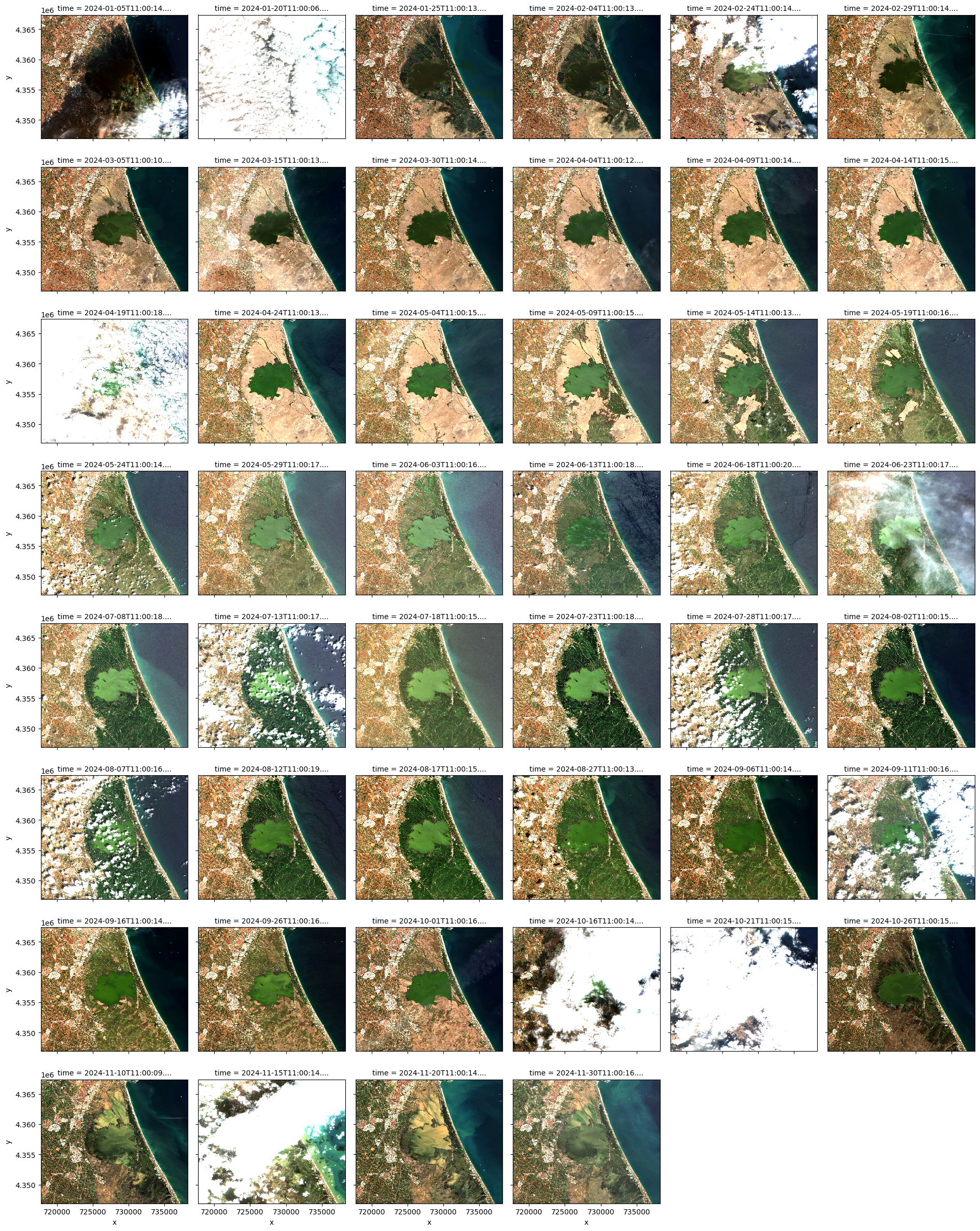
Visualize the retrieved results#
stack.sel(band=["red", "green", "blue"]).plot.imshow(
    row="time", rgb="band", vmin=0, vmax=2000, col_wrap=6
)
<xarray.plot.facetgrid.FacetGrid at 0x128fac590>
Compute NDVI#
# Get bands then compute NDVI
stack = stackstac.stack(
    items,
    bounds=bounds,
    snap_bounds=False,
    epsg=int(epsg.split(":")[-1]),
    resolution=gsd,
    dtype="float64",
    rescale=False,
    fill_value=0,
    assets=["red", "nir"],  # Only need red and nir bands for NDVI
    resampling=Resampling.nearest,
)

# Compute the stack
stack = stack.compute()

# stack shape: (time, band, y, x)
# Get band indexes
red_index = list(stack.band.values).index("red")
nir_index = list(stack.band.values).index("nir")

# Extract bands
red = stack.sel(band="red")
nir = stack.sel(band="nir")

# Compute NDVI
ndvi = (nir - red) / (nir + red + 1e-10)  # small value to avoid division by zero

# Optionally: name the band
ndvi.name = "NDVI"
ndvi_ds = xr.Dataset({"NDVI": ndvi})
print(ndvi_ds)
<xarray.Dataset> Size: 2GB
Dimensions:                                  (time: 46, x: 2048, y: 2048)
Coordinates: (12/49)
  * time                                     (time) datetime64[ns] 368B 2024-...
    id                                       (time) <U24 4kB 'S2B_30SYJ_20240...
  * x                                        (x) float64 16kB 7.178e+05 ... 7...
  * y                                        (y) float64 16kB 4.367e+06 ... 4...
    earthsearch:boa_offset_applied           bool 1B True
    s2:product_type                          <U7 28B 'S2MSI2A'
    ...                                       ...
    view:sun_elevation                       (time) float64 368B 26.3 ... 27.97
    raster:bands                             object 8B {'nodata': 0, 'data_ty...
    gsd                                      int64 8B 10
    proj:shape                               object 8B {10980}
    proj:transform                           object 8B {0, 4400040, 10, -10, ...
    epsg                                     int64 8B 32630
Data variables:
    NDVI                                     (time, y, x) float64 2GB 0.3465 ...
# Compute NDVI at once using stackstac
stack = stackstac.stack(
    items,
    bounds=bounds,
    snap_bounds=False,
    epsg=int(epsg.split(":")[-1]),
    resolution=gsd,
    dtype="float64",
    rescale=False,
    fill_value=0,
    assets=["red", "nir"],  # Only red and NIR bands for NDVI
    resampling=Resampling.nearest,
)

# Extract bands by name
red = stack.sel(band="red")
nir = stack.sel(band="nir")

# Compute NDVI safely
ndvi = (nir - red) / (nir + red + 1e-10)  # small value avoids division by 0

ndvi = ndvi.compute()

# Create a dataset
ndvi.name = "NDVI"
ndvi_ds = xr.Dataset({"NDVI": ndvi})

print(ndvi_ds)
<xarray.Dataset> Size: 2GB
Dimensions:                                  (time: 46, x: 2048, y: 2048)
Coordinates: (12/49)
  * time                                     (time) datetime64[ns] 368B 2024-...
    id                                       (time) <U24 4kB 'S2B_30SYJ_20240...
  * x                                        (x) float64 16kB 7.178e+05 ... 7...
  * y                                        (y) float64 16kB 4.367e+06 ... 4...
    instruments                              <U3 12B 'msi'
    processing:software                      object 8B {'sentinel2-to-stac': ...
    ...                                       ...
    s2:thin_cirrus_percentage                (time) float64 368B 11.14 ... 0.124
    proj:shape                               object 8B {10980}
    raster:bands                             object 8B {'nodata': 0, 'data_ty...
    proj:transform                           object 8B {0, 4400040, 10, -10, ...
    gsd                                      int64 8B 10
    epsg                                     int64 8B 32630
Data variables:
    NDVI                                     (time, y, x) float64 2GB 0.3465 ...
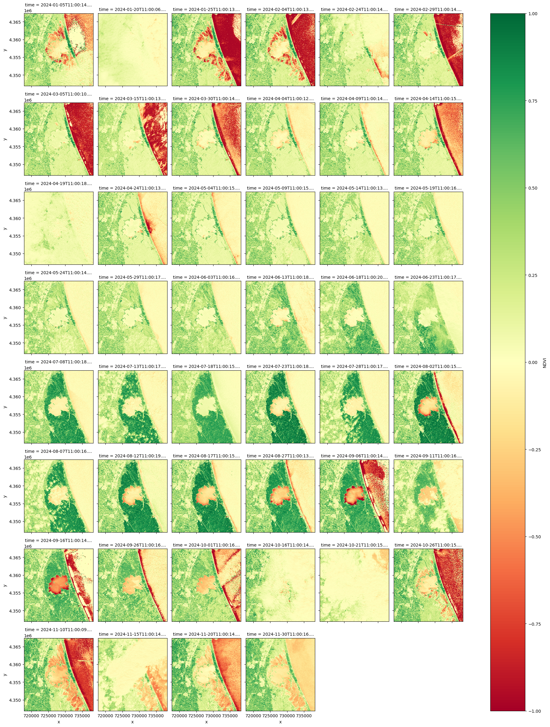
Visualize the NDVI#
ndvi.plot.imshow(
    row="time",
    cmap="RdYlGn",
    vmin=-1,
    vmax=1,
    col_wrap=6,
)
<xarray.plot.facetgrid.FacetGrid at 0x16850ee90>