Download Sentinel-1 Data from Planetary Computer STAC Catalouge

Download Sentinel-1 Data from Planetary Computer STAC Catalouge#

Notebook Description#

This Jupyter Notebook demonstrates how to download and process Sentinel-1 SAR (Synthetic Aperture Radar) data from the Planetary Computer STAC Catalogue. The notebook provides a step-by-step guide to querying, retrieving, and visualizing geospatial data using the stackstac library.

Key Steps#

Library Imports:
- Utilizes libraries such as pystac_client, stackstac, geopandas, shapely, rasterio, planetary_computer, and matplotlib for geospatial data processing and visualization.
API Initialization:
- Connects to the Planetary Computer STAC Catalogue and retrieves an authentication token for secure access.
Data Search:
- Queries the Sentinel-1 RTC (Radiometric Terrain Corrected) collection for SAR imagery based on spatial (bounding box), temporal (date range), and orbit state filters.
Bounding Box Creation:
- Creates a bounding box around a point of interest and reprojects it to the appropriate coordinate reference system (CRS).
Datacube Retrieval:
- Uses the stackstac library to retrieve and process the datacube, specifying desired bands (e.g., VV and VH), resolution, and resampling methods.
SAR Data Conversion:
- Converts SAR backscatter intensity values to logarithmic scale (dB) for better visualization and analysis.
Visualization:
- Visualizes the VV and VH bands of the SAR data as grayscale images for visual inspection.

Import the required libraries#

import geopandas as gpd
import numpy as np
import pandas as pd
import pystac_client
import stackstac
import rasterio
from rasterio.enums import Resampling
from pyproj import Transformer
from shapely import Point
import xarray as xr
import planetary_computer
import requests
from matplotlib import pyplot as plt

Define the URLs and collection name#

TOKEN_URL = "https://planetarycomputer.microsoft.com/api/sas/v1/token"
STAC_API = "https://planetarycomputer.microsoft.com/api/stac/v1"
COLLECTION = "sentinel-1-rtc"

Search the Sentinel-1 Collection#

lat, lon = 39.3336, -0.3545
start = "2024-09-25"
end = "2024-12-01"
# response = requests.get(f"{TOKEN_URL}/{COLLECTION}")

# if response.status_code == 200:
#     response = response.json()
#     token = response["token"]
#     headers ={"Authorization":f"Bearer {token}"}
# else:
#     print(f"Failed to get token. Status code: {response.status_code}")
#     exit()

# Search the catalogue
catalog = pystac_client.Client.open(STAC_API,modifier=planetary_computer.sign_inplace)
# catalog = pystac_client.Client.open(STAC_API)
search = catalog.search(
    collections=[COLLECTION],
    datetime=f"{start}/{end}",
    bbox=(lon - 1e-3, lat - 1e-3, lon + 1e-3, lat + 1e-3),
    )
all_items = search.get_all_items()
items = []
dates = []
for item in all_items:
    if item.datetime.date() not in dates  and item.properties["sat:orbit_state"]=="ascending":
        items.append(item) # when modifier is set, items are signed automatically
        #items.append(planetary_computer.sign_item(item)) # when modifier is not set, items need to be signed manually
        dates.append(item.datetime.date())

print(f"Found {len(items)} items")

/Users/syam/virtualenvs/myvenv/lib/python3.13/site-packages/pystac_client/item_search.py:896: FutureWarning: get_all_items() is deprecated, use item_collection() instead.
  warnings.warn(

Found 10 items

Create bounding box around the point#

# Extract coordinate system from first item
epsg = items[0].properties["proj:code"]

# Convert point of interest into the image projection
# (assumes all images are in the same projection)
poidf = gpd.GeoDataFrame(
    pd.DataFrame(),
    crs="EPSG:4326",
    geometry=[Point(lon, lat)],
).to_crs(epsg)

coords = poidf.iloc[0].geometry.coords[0]

# Create bounds in projection
size = 2048
gsd = 10
bounds = (
    coords[0] - (size * gsd) // 2,
    coords[1] - (size * gsd) // 2,
    coords[0] + (size * gsd) // 2,
    coords[1] + (size * gsd) // 2,
)

Retrieve the pixel values, for the bounding box in the target projection. In this example we use only the RGB and NIR bands.#

stack = stackstac.stack(
    items,
    bounds=bounds,
    snap_bounds=False,
    epsg=int(epsg.split(":")[-1]),
    resolution=gsd,
    dtype="float64",
    rescale=False,
    # fill_value=np.nan,
    assets=["vv","vh"],
    resampling=Resampling.nearest,
)

print(stack)

stack = stack.compute()

<xarray.DataArray 'stackstac-4f4e03a977df621fefe7477875cfbe3e' (time: 10,
                                                                band: 2,
                                                                y: 2048, x: 2048)> Size: 671MB
dask.array<fetch_raster_window, shape=(10, 2, 2048, 2048), dtype=float64, chunksize=(1, 1, 1024, 1024), chunktype=numpy.ndarray>
Coordinates: (12/39)
  * time                                   (time) datetime64[ns] 80B 2024-09-...
    id                                     (time) <U66 3kB 'S1A_IW_GRDH_1SDV_...
  * band                                   (band) <U2 16B 'vv' 'vh'
  * x                                      (x) float64 16kB 2.006e+05 ... 2.2...
  * y                                      (y) float64 16kB 4.369e+06 ... 4.3...
    sat:relative_orbit                     (time) int64 80B 103 30 ... 103 30
    ...                                     ...
    s1:total_slices                        (time) <U2 80B '19' '20' ... '20'
    sar:pixel_spacing_range                int64 8B 10
    raster:bands                           object 8B {'nodata': -32768, 'data...
    description                            (band) <U173 1kB 'Terrain-correcte...
    title                                  (band) <U41 328B 'VV: vertical tra...
    epsg                                   int64 8B 32631
Attributes:
    spec:        RasterSpec(epsg=32631, bounds=(200624.10795189947, 4348925.7...
    crs:         epsg:32631
    transform:   | 10.00, 0.00, 200624.11|\n| 0.00,-10.00, 4369405.78|\n| 0.0...
    resolution:  10

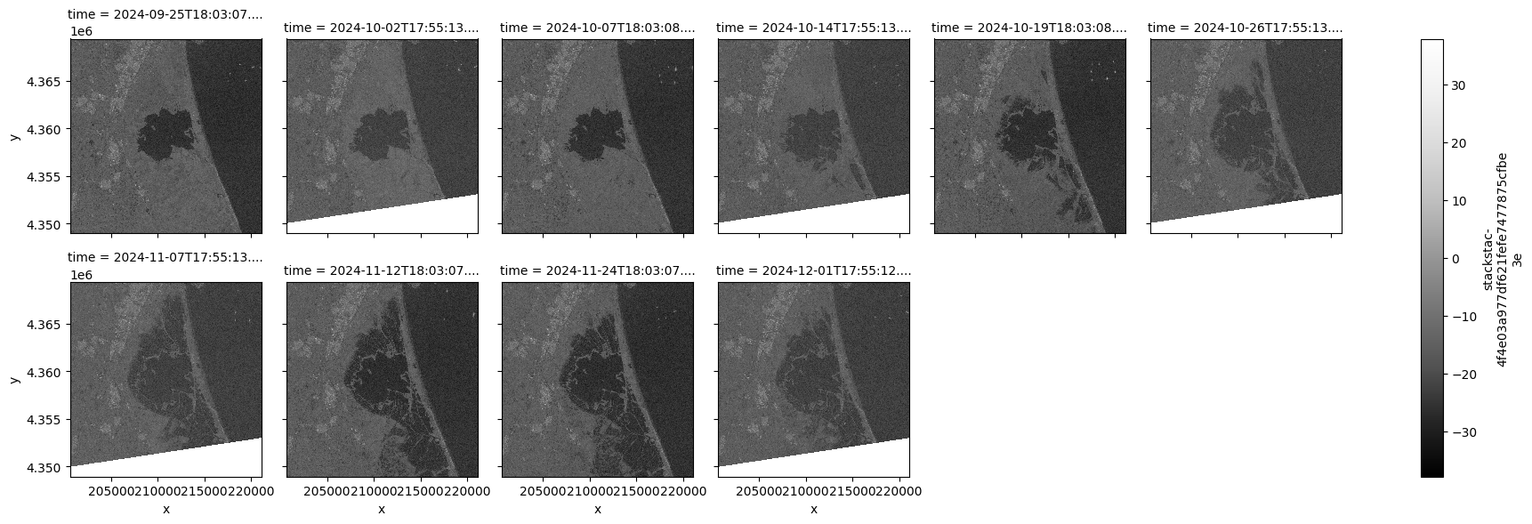
Visualize the VH and VV of the results#

print("VV Band range:", stack_db.sel(band="vv").min().values, stack.sel(band="vv").max().values)
print("VH Band range:", stack_db.sel(band="vh").min().values, stack.sel(band="vh").max().values)
stack_db.sel(band="vv").plot.imshow(
    row="time",
    #vmin=0,
    #vmax=0.6,
    col_wrap=6,
    cmap=plt.cm.Greys_r
)

# Plot VH Band with its own scaling
stack_db.sel(band="vh").plot.imshow(
    row="time",
    #vmin=0,
    #vmax=0.3,
    col_wrap=6,
    cmap=plt.cm.Greys_r
)

plt.show()

VV Band range: -32.76843915565348 1448.4788818359375
VH Band range: -37.85670145810896 232.5352783203125

../_images/2b3285a0cb76ab7ea9d6cfaa624b443d532e47e94f6e4e4bd075aff3458f2692.png

../_images/23c06894684539e10b9167e39966b5d0430eca6ccbe31cd01b782afc2734c041.png